what is the variable use to make a prediciton in data analysis

Creating Regression Models to Predict Information Responses

Learn to create and lawmaking a regression model from scratch to forecast/predict outcomes

Photo past Kelly Sikkema on Unsplash

Regression assay tin can be described as a statistical technique used to predict/forecast values of a dependent variable (response) given values of one or more independent variables (predictors or features). Regression is considered a form of supervised machine learning; this is an algorithm that builds a mathematical model to determine a relationship between inputs and desired outputs. There are numerous regression models that can be generated, so permit's cover regression mathematics first and then jump into 3 mutual models.

Regression Mathematics

Earlier nosotros look at whatever lawmaking, we should understand a little nigh the math behind a regression model. Every bit mentioned, regression models can have multiple input variables, or features, simply for this article, we volition apply a single feature for simplicity. Regression analysis involves making a guess at what blazon of office would fit your dataset the best, whether that be a line, an nth degree polynomial, a logarithmic function, etc. Regression models assume the dataset follows this form:

Here, x and y are our feature and response at observation i, and due east is an error term. The goal of the regression model is to gauge the function, f, and then that it almost closely fits the dataset (neglecting the error term). The office, f, is the guess we make most what type of function would best fit our dataset. This will become more articulate every bit we get to the examples. To approximate the function, nosotros need to estimate the β coefficients. The most common method is ordinary least squares, which minimizes the sum of squared errors betwixt our dataset and our function, f.

Minimizing the squared errors volition consequence in an estimate of our β coefficients, labeled as β-chapeau. The gauge can be obtained using the normal equations that effect from the ordinary least squares method:

In plough, we tin utilise these estimated β coefficients to create an estimate for our response variable, y.

The y-hat value hither is the predicted, or forecasted, values for an observation, i. The prediction is generated past using our estimated β coefficients and a feature value, 10.

To determine how well our regression model performs, we can calculate the R-squared coefficient. This coefficient evaluates the scatter of the dataset effectually the regression model prediction. In other words, this is how well the regression model fits the original dataset. Typically, the closer the value is to 1.0, the better the fit.

To properly evaluate your regression model, yous should compare R-squared values for multiple models (the function, f) before settling on which to use for forecasting hereafter values. Permit's start coding to amend understand the concepts of regression models.

Importing Libraries

For these examples, nosotros will demand the following libraries and packages:

• NumPy is used to create numerical arrays (defined equally np for ease of calling)
• random from NumPy is used to create dissonance in a office to simulate a real-world dataset
• pyplot from matplotlib is used to display our data and trendlines

          # Importing Libraries and Packages
import numpy as np
from numpy import random
import matplotlib.pyplot equally plt        

Creating and Displaying Examination Dataset

To create the dataset, we tin create an ten assortment that will be our feature and a y array that will be our response. The y array is an capricious exponential function. Using the random package, we will introduce noise into our data to simulate some kind of real-world data.

          # Creating Data
10 = np.linspace(0, 4, 500)  # due north = 500 observations
random.seed(10)  # For consistent results run-to-run
noise = np.random.normal(0, 1, ten.shape)
y = 0.25 * np.exp(x) + noise
# Displaying Data
fig = plt.figure()
plt.scatter(x, y, south=3)
plt.title("Test Data")
plt.xlabel("ten")
plt.ylabel("y")
plt.evidence()
                  

Here is the dataset that nosotros apply regression analysis to:

Examination Data [Created by Author]

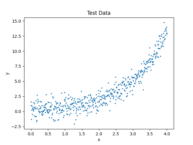
Let's have a second to look at this plot. We know that an exponential equation was used to create this information, but if we did not know that information (which you wouldn't if you are performing regression assay), nosotros might look at this information and remember a 2d degree polynomial would fit the dataset the best. Withal, equally best practice, you lot should evaluate a couple unlike models to see which performs the best. And so, you volition use the all-time model to create your predictions. At present let's wait at a couple regression models separately and meet how their results compare.

Linear Regression

Every bit mentioned in the mathematics section, for regression analysis you guess a model, or function. For a linear model, the post-obit form is taken for our role, f:

The adjacent pace is creating the matrices for the normal equations (in the mathematics section) that approximate our β coefficients. They should look like the following:

Using our dataset, our estimated β coefficients and therefore linear regression model will be:

          # Linear Regression
X = np.array([np.ones(x.shape), x]).T
X = np.reshape(X, [500, 2])
# Normal Equation: Beta coefficient approximate
b = np.linalg.inv(10.T @ X) @ Ten.T @ np.array(y)
print(b)
            
# Predicted y values and R-squared
y_pred = b[0] + b[one] * x
r2 = 1 - sum((y - y_pred) ** ii)/sum((y - np.mean(y)) ** 2)
            
# Displaying Data
fig = plt.figure()
plt.besprinkle(x, y, south=3)
plt.plot(ten, y_pred, c='ruby')
plt.championship("Linear Model (R$^2$ = " + str(r2) + ")")
plt.xlabel("x")
plt.ylabel("y")
plt.legend(["Data", "Predicted"])
plt.evidence()
                  

The resulting regression model is shown below:

Test Data [Created by Author]

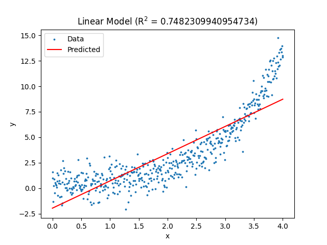
Equally you tin can run across in the title of the plot, the linear regression model has an R-squared value of virtually 0.75. This means the linear model fits the data okay, only if we were to collect more data, we would likely meet the value of R-squared decrease substantially.

Polynomial Regression

The general form of polynomial regression is equally follows:

This commodity shows the form of the role, f, equally a second order polynomial. You lot tin can add more than polynomial terms in a similar manner to fit your needs; still, be wary of overfitting.

Creating the matrices for the normal equations gives the post-obit:

Using these matrices, the estimated β coefficients and polynomial regression model will exist:

          # Polynomial Regression
X = np.assortment([np.ones(x.shape), x, 10 ** 2]).T
X = np.reshape(Ten, [500, iii])
# Normal Equation: Beta coefficient approximate
b = np.linalg.inv(X.T @ X) @ X.T @ np.assortment(y)
print(b)
            
# Predicted y values and R-squared
y_pred = b[0] + b[1] * ten + b[two] * x ** two
r2 = 1 - sum((y - y_pred) ** ii)/sum((y - np.mean(y)) ** two)
            
# Displaying Data
fig = plt.figure()
plt.scatter(x, y, south=3)
plt.plot(x, y_pred, c='cerise')
plt.title("2$^{nd}$ Degree Poly. Model (R$^2$ = " + str(r2) + ")")
plt.xlabel("x")
plt.ylabel("y")
plt.fable(["Data", "Predicted"])
plt.bear witness()
                  

The resulting plot:

Test Information [Created by Writer]

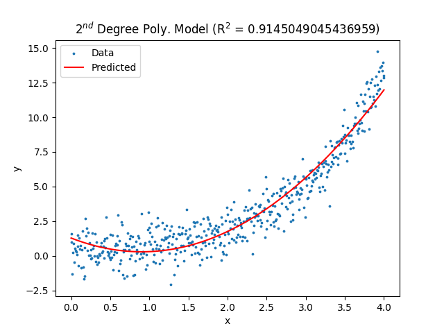
Detect the 2nd degree polynomial does a much ameliorate chore of matching the dataset and achieves an R-squared value of about 0.91. Notwithstanding, if nosotros expect towards the end of the dataset, nosotros notice the model is underpredicting those information points. This should encourage us to look into other models.

Exponential Regression

If we decided confronting the polynomial model, our side by side choice could be an exponential model of the grade:

Once again, creating the matrices for the normal equations gives the following:

At present, with the estimated β coefficients, the regression model will be:

Note that the leading coefficient on the exponential term closely matches the simulated data leading coefficient.

          # Exponential Regression
X = np.assortment([np.ones(x.shape), np.exp(x)]).T
X = np.reshape(Ten, [500, two])
# Normal Equation: Beta coefficient gauge
b = np.linalg.inv(X.T @ 10) @ X.T @ np.array(y)
print(b)
            
# Predicted y values and R-squared
y_pred = b[0] + b[ane]*np.exp(x)
r2 = i - sum((y - y_pred) ** ii)/sum((y - np.mean(y)) ** 2)
            
# Displaying Data
fig = plt.figure()
plt.scatter(ten, y, south=3)
plt.plot(10, y_pred, c='red')
plt.championship("Exponential Model (R$^2$ = " + str(r2) + ")")
plt.xlabel("x")
plt.ylabel("y")
plt.fable(["Data", "Predicted"])
plt.show()
                  

The resulting effigy:

Test Data [Created past Author]

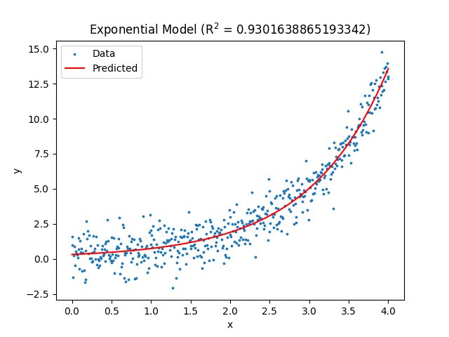
Notice in that location is improvement in the R-squared value compared to the 2d degree polynomial model. Fifty-fifty more promising is the end of the dataset fits this model better than the second degree polynomial. Given that information, we should use the exponential model to predict hereafter y values for the well-nigh accurate upshot possible.

That wraps up the article. Hopefully this gives you an idea of how regression analysis can be performed in Python and how to use it properly for real-earth scenarios. If yous learned something, requite me a follow and check out my other articles on space, mathematics, and Python! Thank you lot!

barnhartfashe1978.blogspot.com

Source: https://towardsdatascience.com/creating-regression-models-to-predict-data-responses-120b0e3f6e90

Share this post